8. Estimating the Risks
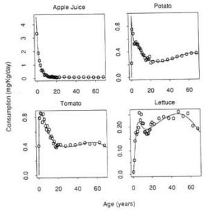
THE PRECEDING CHAPTERS have demonstrated that infants and children may have special sensitivities to certain toxic insults. Children also consume notably more of certain foods relative to their body weight than do adults. Thus, their ingestion of pesticide residues on these foods may be proportionately higher than that of adults. For certain chronic toxic effects such as cancer, exposures occurring early in life may pose greater risks than those occurring later in life. For these reasons, risk assessment methods that have traditionally been used for adults may require modification when applied to infants and children.
To evaluate the potential risks from dietary intake of pesticide residues by infants and children, some familiarity with basic toxicological approaches to risk assessment is required. In the first part of this chapter, the committee reviews principles of toxicological risk assessment, including interspecies extrapolation, forms of toxicity, mathematical models for assessing cancer risk, low-dose linearity, and multiple exposures. Special characteristics of infants and young children that must be considered when assessing their risks from dietary exposures to pesticides are then discussed.
The fundamental purpose of regulatory toxicology is the determination of risks (including zero risk) at various possible levels of human exposure to toxicants present in the environment. For risk assessment applications, it is useful to distinguish between toxic processes that are either stochastic or nonstochastic in nature. Stochastic processes such as carcinogenesis result from the random occurrence of one or more biological events in specific individuals. Thus, whether or not a particular individual will develop a cancerous lesion under specified conditions or exposure cannot be predicted with certainty. Nonstochastic events such as enzyme inhibition following exposure to a certain toxicant are more predictable. Nonstochastic effects may not be seen if lifetime exposures are below a certain threshold concentration, whereas stochastic effects such as carcinogenesis may have no threshold. Different approaches to risk assessment are usually used for these two categories of response.
Information on health risks may be obtained directly from epidemiological and other studies of humans or indirectly through toxicological experiments conducted in animal models. Although results of laboratory studies are applicable to humans only indirectly, they can be used to predict potential health hazards in advance of actual human exposure and thus continue to be used widely to identify substances with potential toxicity.
Three major problems are inherent in the translation of results of animal tests to humans:
• Laboratary tests are conducted at relatively high doses to induce measurable rates of response in a small sample of animals. These results must often extrapolated to lower doses that correspond to anticipated human exposure levels.
• Interspecies differences must be considered when extrapolating between the animal model and humans.
• It may be necessary to extrapolate from a route of exposure chosen for experimental practicality to a different but more likely route of human exposure.
General Principles of Risk Assessment
Toxicological Risk Assessment
Classical methods in toxicological risk assessment are applicable with nonstochastic toxic effects. For many kinds of agents and end points, toxicity is manifest only after the depletion of a physiological reserve. In addition, the biological repair capacity of many tissues can accommodate a certain degree of damage by reversible toxic processes (Aldridge, 1986; Klaassen, 1986). Above this threshold, however, the compensatory mechanisms that maintain normal biological function may be overwhelmed, leading to organ dysfunction. The objective of classical toxicological risk assessment, which has focused on nonstochastic end points, has been to establish a threshold dose below which adverse health effects were expected to be rare or absent.
Historically, the threshold concept was introduced by Lehman and Fitzhugh (1954), who proposed that an acceptable daily intake (ADI) could be calculated for chemical contaminants in human food. This concept was endorsed by the Joint FAO/WHO Expert Committee on Food Additives (JECFA) in 1961 and subsequently adopted by the Joint FAO/WHO Meeting of Experts on Pesticide Residues (JMPR) in 1962 (Lu, 1988). Formally, the ADI was defined as:
ADI = NOEL/SF,
where the NOEL is the no-observed-effect level in toxicity studies, usually in the most sensitive species, and SF is the safety factor. Weight loss, reduction in weight gain, alteration in organ weight, and inhibition of cholinesterase activity are indicative of specific adverse effects that may be considered when establishing the NOEL (Babich and Davis, 1981). The safety factor makes allowances for the type of effect, the severity or reversibility of the effect, and variability among and within species (NRC, 1970).
In 1977, the National Research Council's Safe Drinking Water Committee reviewed the methods that had evolved for establishing ADIs and made several important recommendations. First, the committee proposed that the NOEL be expressed in mg/kg of body weight rather than mg/kg of diet to adjust for differences in dietary consumption patterns. Since children consume proportionally more food relative to body weight than do adults, ADIs established on a body weight basis would be more protective of children than would ADIs established as dietary concentrations. Second, the committee explicitly supported the use of only a 10-fold safety factor (now called uncertainty factor) in the presence of adequate dose-response data derived from human studies. And third, the committee proposed an additional 10-fold safety factor in the absence of adequate toxicity data, for an overall safety factor of 100. The use of these factors was later supported in a report by the Safe Drinking Water Committee in a reexamination of the earlier risk assessment practices (NRC, 1986). For carcinogenesis, that committee proposed the following definitions for two levels of safety factors:
• 10: When studies in humans involving prolonged ingestion have been conducted with no indication of carcinogenicity.
• 100: When chronic toxicity studies have been conducted in one or more species with no indication of carcinogenicity. Data on humans are either unavailable or scanty.
With cholinesterase inhibitors, an uncertainty factor of 10 is applied, since toxicity in humans and animals has been shown to be similar, and because the effect is generally reversible. An uncertainty factor of 100 is more commonly used for compounds with other toxic end points, assuming that humans are 10 times more sensitive than the most sensitive test animal and that the most sensitive humans are 10 times more sensitive than the average human. The interspecies uncertainty factor is based on studies in adult laboratory animals and, therefore, is applicable to adult human beings, but studies in adult laboratory animals are not necessarily good for predicting the response of human infants and children. The other 10-fold intraspecies uncertainty factor is meant to cover variations within human populations, including genetic predisposition, poor nutrition, disease status, and age (Babich and Davis, 1981). A factor of 10 for intraspecies variation in susceptibility may be sufficient for any one element of interpersonal difference but may not be sufficient for multiple elements. Thus, as presently determined, an uncertainty factor of 100 may not be sufficient to account for the potential increased sensitivity of infants and children.
When insufficient toxicity data are available, an uncertainty factor of 1,000 may be applied. The ADI is then converted to the maximal permitted intake (MPI), which is the product of the ADI and the average body weight of an adult, considered to be 60 kg, or sometimes 70 kg, by the U.S. Environmental Protection Agency (EPA) and 70 kg by the Food and Drug Administration (FDA) (Babich and Davis, 1981).
Uncertainty factors used in toxicological risk assessment have some widely recognized limitations. Since the ADI is based on an estimate of the population threshold or true no-effect level (NEL), it does not provide absolute assurance of safety (Crump, 1984b). Larger and better studies can demonstrate effects at lower doses, but the size of the uncertainty factor is not directly related to sample size. Therefore, smaller and poorer experiments tend to lead to larger ADIs (Schneiderman and Mantel, 1973). Although a factor of 10 is used to accommodate variation in sensitivity among species, and another factor of 10 is used for variation within a species, it cannot be guaranteed that a combined uncertainty factor of 100 will afford adequate protection in all cases. Nor are these factors of 10 based on validated biological models. There is additional uncertainty, usually small, about whether some observed biological responses are adverse effects or innocuous. Thus, the ADI is not intended to have a high degree of mathematical precision. Rather, it is a guide to human exposure levels that are not expected to present serious health risks.
The EPA has recommended using the term uncertainty factor (UF) rather than safety factor in recognition of the fact that the ADI does not guarantee absolute safety consistent with more recent recommendations of the Safe Drinking Water Committee (NRC, 1986). The agency has also adopted the reference dose (RfD) as a replacement for the ADI (Barnes and Dourson, 1988; EPA, 1988). In addition, EPA introduced the concept of a modifying factor (MF) to be applied to the UF in recognition of the possible special circumstances surrounding the establishment of a specific RfD. The RfD is determined by use of the equation:
RfD = NOAEL/(UF x MF),
where the NOAEL (no-observed-adverse-effect level) is the highest dose at which there is no statistically significant adverse effect in the test animals beyond that exhibited by a control group, and the UF accommodates uncertainties in the extrapolation of dose-threshold data to humans. The MF is applied when scientific uncertainties in the study are not accommodated by the UF. When the data do not demonstrate a NOAEL, a LOAEL (lowest-observed-adverse-effect level) may be used. This is the lowest dose at which a statistically significant adverse effect is observed.
The NOAEL and the LOAEL depend on the design of the study, particularly on the selection of the experimental dose groups. If the dose groups are far apart, then the LOAEL may be significantly higher than the true concentration at which adverse effects occur and the NOAEL may be much lower than the minimum concentration producing an adverse effect. In the present context, the term adverse effect is defined as any effect that results in a functional impairment or pathological lesion that may affect the performance of the whole organism, or that reduces the ability of the organism to respond to additional challenges (Dourson, 1986).
By definition, a UF is a number that reflects the degree of uncertainty that must be considered when experimental data are extrapolated to humans (Dourson and Stara, 1983; Barnes and Dourson, 1988). When the critical study (the one with the best available dose-response data) is selected for calculation of the reference dose, five factors may contribute to the composite uncertainty factor:
• the need to extrapolate from animal data to humans when human exposure data are unavailable or inadequate;
• the need to accommodate human response variability to include sensitive subgroups;
• the nature, severity, and chronicity of the effect;
• the need to accommodate the necessity of using LOAEL rather than NOAEL data; and
• the need to extrapolate from a data base that is inadequate or incomplete.
The overall UF may vary from 1 to 10,000, depending on the combination of these individual factors, but usually does not exceed 100. An MF between 1 and 10 may be used to account for scientific uncertainties, either in the study or in the data base, that are not explicitly taken into consideration in any of the five factors listed above (Barnes and Dourson, 1988). For example, application of the MF may be regarded as a professional judgment that each test group contained too few animals.
Cancer Risk Estimation
The quantitative estimation of risks associated with low levels of exposure to carcinogens present in the environment is an important part of the regulatory process. At present, risk estimation methods are usually based on the assumption that the dose-response curve for carcinogenesis is linear in the low-dose region. This position is reflected in the principles proposed by the Office of Science and Technology Policy (1986), which stated:
When data and information are limited … and when much uncertainty exists regarding the mechanism of carcinogenic action, models or procedures which incorporate low-dose linearity are preferred. (OSTP, 1986)
This position is also reflected in the EPA's (1986) Carcinogen Risk Assessment Guidelines.
Although the Guidelines emphasize risk estimates derived using some form of linear extrapolation, they are based on the assumption that such estimates may be more appropriately viewed as plausible upper limits on risk and that the lower limit may well be effectively zero. The Guidelines also state that procedures for obtaining a best estimate lying somewhere between these two extremes generally do not exist at present, but that it may be possible to move away from a linearized extrapolation to obtain an upper limit in some circumstances and instead, use a threshold approach. For example, the EPA has recently taken a step in this direction by considering the possibility of a threshold for the induction of thyroid tumors (Paynter et al., 1988).
The EPA now uses the linearized multistage model for low-dose cancer risk estimation. The most important aspect of this practice is not the choice of the multistage model itself for risk estimation purposes but, rather, the linearized form of the model. Because the model is constrained to be linear at low doses, it is expected to yield risk estimates comparable to those based on other linear extrapolation procedures, including those proposed by Gaylor et al. (1987) and Krewski et al. (1990).
Additivity to Background and Low-Dose Linearity
Additivity to background is often cited in support of the assumption of low-dose linearity in carcinogenic risk assessment. In the additive background model proposed by Crump et al. (1976) and Peto (1978), spontaneous tumors are associated with an effective background dose, to which exposure from environmental carcinogens is added. According to Crump and colleagues:
If carcinogenesis by an external agent acts additively with an already ongoing process, then under almost any model the response will be linear at low doses. (Crump et al., 1976)
Hoel (1980) subsequently demonstrated that this result also holds for partial additivity. This is expressed as follows in the current Guidelines:
If a carcinogenic agent acts by accelerating the same carcinogenic process that leads to the background occurrence of cancer, the added effect of the carcinogenic process at low doses is expected to be virtually linear. (EPA, 1986)
The basic idea behind the additive background model is illustrated in Table 8-1. Here the spontaneous response rate is considered to arise as a consequence of a background dose d, and the effects of the test chemical administered at dose d are additive in a dosewise fashion. The linearity of the excess risk over background P(d + d) - P(d) at low doses follows from the fact that the secant between doses of d and (d + d) converges to the tangent to the dose-response curve as the dosed of the test compound becomes small.
Within the framework of this model, the only condition required for this result to hold is that the probability of tumor occurrence be a smooth, strictly increasing function of dose. No further assumptions are required concerning either the mathematical form of the dose-response relationship or the toxicological mechanism by which tumors are induced.
The low-dose linearity implied by this model refers to the slope of the dose-response curve at an applied dose of zero. Without additional assumptions, no further general statements can be made about the magnitude of this slope or about the range of low doses over which this linear approximation will be sustained reasonably well. The linear approximation in the multistage model holds well, even at doses that double the background tumor rate if that rate is not trivially small (Crump et al., 1976). When attempting to fit curves in the average regulatory setting, however, the lowest dose tested under usual experimental conditions is often one-quarter or a smaller fraction of the MTD (NRC, 1993). Compared to actual dietary concentrations, one-quarter of the MTD will often be very high, and linear interpolation between a tumor response at one-quarter or less of the MTD and the tumor response of the controls may still overestimate the response at the (low) regulatory dose and the low dose to which it is anticipated that humans will be exposed.
TABLE 8-1 Effect of Background Rate on Accuracy of Additivity Approximation Under the Assumption of the Multistage Modela
a From NRC, 1988, p. 196.
Nonlinearity at High Doses
Linearity at low doses does not imply that the dose-response curve will also be linear at high doses. In particular, curvature at high doses can result from factors such as saturation of absorption or elimination pathways or the alteration of pharmacokinetic processes involved in metabolic activation (Hoel et al., 1983). Nonlinearity at high doses can also be attributable to saturation of DNA repair systems or the induction of cellular proliferation. Dose-response curves for chemicals that can both cause DNA damage and induce cellular proliferation can be subject to a high degree of upward curvature, as with the hockey-stick-shaped dose-response curves for tumors of the urinary bladder induced by 2-acetylaminofluorene (2-AAF) (Cohen and Ellwein, 1990). Similarly, secondary carcinogens may act only at relatively high doses.
Nonlinearity due to saturation of elimination pathways results in upward curvature (as with methylene chloride), whereas saturation of activation processes leads to downward curvature (as with vinyl chloride). For processes that saturate in accordance with Michaelis-Menten kinetics, however, the amount of the proximate carcinogen formed at low doses will be directly proportional to the administered dose, since such processes are essentially first order at low doses (Murdoch et al., 1987). But again there is no way to estimate the shape or the range of the linearity.
If the pharmacokinetic model governing metabolic activation is known, dose-response may be assessed in terms of the dose delivered to the target tissue (NRC, 1987a). This may result in a more nearly linear dose-response curve, which greatly facilitates statistical extrapolation to low doses (Hoel et al., 1983; Krewski et al., 1986). To estimate delivered dose, however, it is important to consider the uncertainty associated with the parameters used in the pharmacokinetic model (Portier and Kaplan, 1989). Several additional parameters introduced in the modeling when pharmacokinetics is considered will introduce more uncertainty.
Molecular Dosimetry
Different chemicals may induce different kinds of DNA lesions involving anywhere from two to 13 sites on molecular DNA (NRC, 1989). At the same time, there is evidence that spontaneously occurring DNA lesions (i.e., those with no known cause) can differ from those caused by exposure to alkylating agents. This suggests that fingerprinting of DNA damage in exposed and unexposed individuals may provide a practical means for distinguishing between additive and independent backgrounds.
The dose-response curve for tumor induction can be linear or nonlinear for a genotoxic agent that acts completely independently of background. If neoplastic conversion can result from a single mutagenic DNA lesion, the linearity of adduct formation at low doses implies linearity with respect to tumor induction (Lutz et al., 1990). If two or more mutagenic lesions are required to create a malignant cancer cell, however, the dose-response curve will be nonlinear with an effective threshold at low doses. This is essentially a multihit, independent background model in which the response is proportional to dose raised to a power equal to the number of DNA lesions required for neoplastic conversion.
Mathematical Modeling of Cancer Risk
Mathematical modeling has been a dominant feature of the quantitation of cancer risk. However, no model has been adequately validated in practice, and none account for all possible situations. Following are brief general descriptions of the more important risk assessment models that have been proposed and used over the years as background for the assessment of the risk to children from dietary exposures to pesticides.
Linear Extrapolation Approaches. In the absence of evidence to the contrary, existing arguments support the adoption of low-dose linearity for cancer risk assessment. Various methods for low-dose linear extrapolation have been proposed by several investigators. Gross et al. (1970) suggested discarding data starting at the highest dose until a linear model provided an adequate description of the remaining data. Van Ryzin (1980) proposed the use of any dose-response model that fits the data reasonably well to estimate the dose producing an excess risk of 1% followed by simple linear extrapolation to lower doses. Gaylor and Kodell (1980) suggested fitting a dose-response model to obtain an upper confidence limit on the probability of tumor incidence at the lowest experimental dose and then using linear extrapolation at doses between zero and that dose. Since estimates at low doses might be unduly influenced by the choice of the dose-response model, Farmer et al. (1982) recommended linear extrapolation below the lowest experimental dose, or from the dose corresponding to an excess risk of 1%, whichever is larger.
Krewski et al. (1984) proposed what is called a model-free procedure using a linear interpolation from the response at the lowest dose showing any increase, down to the response at zero dose (i.e., control response). This approach is simple, but is not strictly model free, since the use of a linear interpolation implies a model of response directly proportional to the dose or exposure. Krewski et al. (1986) modified this procedure to consider the upper confidence limits of the low-dose slopes for each dose showing no statistically significant increase in tumor incidence above background. The shallowest slope was then selected for low-dose risk estimation.
Gaylor (1987) recommended using the smallest upper confidence limit where there is evidence to believe that the lowest dose is in a portion of the dose-response curve that is likely to lie between linearity and some upward curvature. Only rarely is it known with any exactness where this region is located, and often it is not certain that it exists at all.
Because of the difficulties in specifying and implementing a fully biologically based model of carcinogenesis for purposes of risk assessment (NRC, 1993), simple model-free approaches to low-dose risk estimation are attractive, especially when little is known about the process of tumor induction. Krewski et al. (1991) compared the behavior of the upper confidence limits of the slopes obtained from the model-free extrapolation (MFX) procedure with the upper confidence limit of the low-dose slope estimate obtained from the linearized multistage (LMS) procedure of Crump (1984a), as described below in the section on ''Estimates of Carcinogenic Potency." Comparisons were obtained for 572 bioassays taken from a compilation in the Carcinogenic Potency Database by Gold et al. (1984). Bioassays were restricted to rodent experiments exhibiting definite carcinogenicity. The median of the ratio of the upper 95% confidence limits on low-dose slopes for MFX: LMS was 1.3. In 433 of the 572 bioassays, the MFX estimate was within a factor of two of the LMS estimate. In eight cases, the MFX estimate exceeded the LMS estimate by a factor of 10. In these cases, there was a leveling off or decrease in the slope of the dose-response curve at higher doses, which tended to reduce the LMS values.
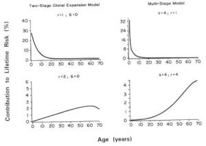
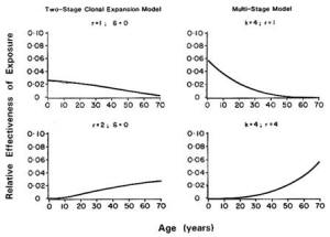
Biologically Based Cancer Models. The multistage model has a long history of use in theoretical descriptions of carcinogenesis (Whittemore and Keller, 1978; Brown and Koziol, 1983; Armitage, 1985). As described by Armitage and Doll (1961), a stem cell must sustain a series of mutations in order to give rise to a malignant cancer cell. This model predicts that the age-specific cancer incidence rates should increase in proportion to age raised to a power related to the number of stages in the model, and provides a good description of many forms of human cancer by allowing for two to six stages.
The biological basis for the multistage model is incomplete in that it does not incorporate tissue growth or cell kinetics. Furthermore, as many as six stages may be required to describe dose-response curves with high upward curvatures, raising questions of biological interpretation. For these reasons, dose-response models that do reflect certain biological processes (e.g., cell deaths, cell turnover) have received considerable attention in recent years. Perhaps most widely discussed is the two-stage mutation-birth-death model, which was developed by Moolgavkar, Venzen, and Knudson and is therefore known as the MVK model (Moolgavkar, 1968a,b).
The MVK model is a biologically motivated model of carcinogenesis based on the hypothesis that a tumor may be initiated following genetic damage in one or more cells in the target tissue as a result of exposure to a compound called an initiator (Moolgavkar, 1986a,b; Thorslund et al., 1987). The initiated cells may then undergo a further transformation to give rise to a cancerous lesion. The rate at which such lesions occur may be increased by subsequent exposure to a promoter, which increases the pool of initiated cells through clonal expansion. Mathematical formulations of this process have been developed by Greenfield et al. (1984) and Moolgavkar et al. (1988).
The MVK model assumes that two mutations are necessary for a normal cell to become malignant. Initiating activity may be quantified in terms of the rate of occurrence of the first mutation. The rate of occurrence of the second mutation quantifies progression to a fully differentiated cancerous lesion. Promotional activity is measured by the difference in the birth and death rates of initiated cells. In the absence of promotional effects and variability in the pool of normal cells, the two-stage mutation-birth-death model reduces to a classic two-stage model.
The MVK model provides a convenient context for the quantitative description of the initiation/promotion mechanisms of carcinogenesis (Moolgavkar, 1986a). As described above, initiator increases the rate of occurrence of the first mutation, whereas a promoter increases the pool of initiated cells. Thus, the term progressor is used to describe an agent that increases the rate of occurrence of the second mutation, resulting in malignant transformation to a cancerous cell (EPA, 1987). It is possible that the same agent could play two or even all three of these roles (initiator, promoter, progressor), thereby enhancing both initiation and progression.
This model was applied by Thorslund and Charnley (1988) in estimating cancer risks associated with exposure to dioxin and chlordane, two putative tumor-promoting agents. The model provided a good fit to laboratory bioassay data on these two compounds, thereby facilitating a quantitative description of the mechanism of carcinogenic action within the framework of the MVK model. Using either a simple exponential (one-hit) or logistic model to describe the dose-response relationship for promotion, these investigators developed estimates of risk that were appreciably lower than those based on the linearized multistage model. Before this model can be recommended for routine application, however, its statistical properties require further study, especially with respect to predictions of risk at low doses (Portier, 1987).
Because the MVK model can be used to describe a variety of dose-response curves, it may not always provide an adequate description of the most important events involved in tumor induction. In certain cases, more than two mutations may be required for neoplastic conversion. Similarly, nongenotoxic factors may be required to foster development of a malignant tissue mass. As additional components are incorporated, the model rapidly becomes more complex and its tractability will be reduced (NRC, 1993).
Despite this potential for further elaboration, the MVK model is viewed as biologically more meaningful than the Armitage-Doll multistage model (Armitage, 1985). To apply this model, however, it will be necessary to have data on tissue growth and cell kinetics as well as bioassay data on tumor occurrence. Attempts to estimate all the parameters involved in the model without such supplementary data may result in unstable estimates (Portier, 1987). Separate estimates of the parameters governing the two mutation rates characterizing the genotoxic process in the model will also require more elaborate bioassay protocols than those currently in use (EPA), 1987). Nonetheless, explorations of the MVK model should be encouraged in order to learn more about its utility (NRC, 1993).
Estimates of Carcinogenic Potency. Several numerical indices have been proposed to describe the potency of chemical carcinogens (Barr, 1985). This concept derives from early work by Twort and Twort (1933) and Iball (1939). Gold et al. (1984) used the results of laboratory studies of carcinogenicity to tabulate the TD50 for a large number of chemical carcinogens, thereby popularizing the TD50 index. The TD50 for carcinogenesis is defined as the dose that reduces the proportion of tumor-free animals by 50% (Peto et al., 1984; Sawyer et al., 1984).
Some correlation has been noted between the TD50 and the LD50 used to measure acute toxicity (Zeise et al., 1984, 1986), although the correlation is not high (Metzger et al., 1989). The TD50 is also highly correlated with the maximum tolerated dose (MTD), which is often used as the high dose in carcinogenicity bioassays (Bernstein et al., 1985). Little correlation between the TD50 and biological indicators of tumor pathology is apparent (Gold et al., 1986), however, indicating the impossibility of summarizing the characteristics of a chemical carcinogen in a single index (Wartenberg and Gallo, 1990).
Correlations between the TD10, LD50, and MTD need to be interpreted with care (Crouch et al., 1987). Since the range of possible values of the TD50 is limited by the choice of the MTD, the wide variation in the carcinogenic potency of different chemicals could produce a correlation between these two indices (Bernstein et al., 1985). In this regard, Rieth and Starr (1989) noted that little correlation exists between the TD50 and MTD after normalizing the TD50 values relative to the MTD. These investigators also suggest that the correlation between the LD50 and the TD50 may increase in part because an observed TD50 could be larger than the LD50.
The TD50 may be of some use in representing the overall strength of carcinogenic substances, but it does not necessarily indicate the level of risk posed at low exposure levels (Wartenberg and Gallo, 1990). As discussed previously, assessment of risk at low doses is generally accomplished by extrapolating results obtained at higher doses approaching the TD50.
As noted above, the EPA (1986) uses the linearized multistage model to estimate risk at low doses. A risk assessment analysis based on the LMS uses q1* (a quantitative carcinogenic potency factor) (Crump, 1984a), which is the estimated slope of the dose-response curve from animal tests yielding a positive carcinogenic response. The q1* value represents the estimated tumor incidence (the number of tumors per milligrams of pesticide per kilogram of body weight per day) at the relatively low concentrations of pesticides found in the human diet. It is based on a mathematical extrapolation of tumor incidence observed at the high doses used in tests in laboratory animals. High and low q1* values indicate strong and weak carcinogenic responses, respectively. For example, q1* values are 9.4 x 10⁻¹ for chlordimeform, 2.3 x 10⁻³ for captan, and 5.9 x 10⁻⁵ for glyphosate (NRC, 1987b). Chlordimeform is thus considered a more potent carcinogen than captan (roughly 30-fold) or glyphosate (roughly 200-fold).
The q1* values among pesticides can vary by orders of magnitude (NRC, 1986, 1987b). The estimated q1* depends on whether a surface area or body weight correction is made in extrapolating risks from rodents to human beings, whether malignant and benign tumors are combined, and the extrapolation model used. The EPA uses surface area, whereas FDA uses body weight.
The EPA follows a policy in setting q1* values that minimizes the chance of underestimating cancer risks. As a result, EPA's estimates derived by using the q1* are believed by many to lead to an overestimate of the cancer risk. Use of the upper 95% confidence limit of the slope of the dose-response curve attempts to allow for variability in response among the laboratory animals and statistical stability in the estimate, and thus possibly errs on the side of caution when extrapolating risk to humans. However, the approach makes no allowance for variability among humans, such as the possible existence of highly susceptible persons, or other sources of uncertainty.
The value of q1* is the slope of the fitted dose-response curve in the low-dose region. It estimates the risk associated with a standard dose (such as 1 mg/kg/day). EPA uses the upper confidence limit on this slope both to introduce caution into its estimates and to provide a more stable measure of risk than would come about if the maximum likelihood (ML) estimate of the slope were used. The ML estimate is highly unstable, and the addition or removal of one or two tumor-bearing animals leads to large swings in the slope estimate and, hence, the risk estimate. The value of q1* derived is negatively correlated with the TD50 (Krewski et al., 1989, 1993). Thus, compounds with a low TD50 will tend to be associated with higher levels of estimated risk at low doses than will compounds with high TD50s.
EPA uses a time-independent model that estimates the lifetime risk of cancer and assumes that the risk from a given dose is the same at all ages. EPA's model assumes, for example, that the excess risk from exposure at age 5 is the same as the risk from the same exposure at age 70. However, because high levels of exposure to carcinogenic pesticides may occur during childhood and because decades may pass before the cancer resulting from that exposure is manifested, the use of EPA's methodology may substantially underestimate the lifetime cancer risk at young ages of exposure.
As noted in Chapter 4 (Methods for Toxicity Testing), the toxicity data base used in either the time-independent or time-dependent models for cancer risk assessment derives from carcinogenicity studies in young adult or adult laboratory animals whose responses may not be representative of those in neonates and weanlings. Newborn animals are often found to be more sensitive to certain carcinogens than are older animals (Rice, 1979). Thus, carcinogenicity studies in young adult animals, as recommended by EPA, may underestimate risks from exposures incurred during infancy or childhood—whether the time-dependent or time-independent models are used.
Species Conversion
In the absence of direct information on the carcinogenic potential of a particular agent in humans, toxicity studies in animals are often used as the basis for carcinogenic risk assessment (Rall et al., 1987). At present, all known human carcinogens have also been shown to be carcinogenic in one or more animal species (IARC, 1987). Although this does not necessarily imply that all compounds that are clearly carcinogenic in animals will also be carcinogenic in humans, it is considered prudent to regard them as such. Empirical support for this position may be derived from the high concordance in results reported as positive and negative (74% when effects in both sexes are considered) between rats and mice exposed to 266 different chemicals tested for carcinogenicity in the U.S. National Toxicology Program (NTP) (Haseman and Huff, 1987). True concordance may be higher but observed only in small samples with imperfect laboratory methods. These same data were used by Chen and Gaylor (1987) to demonstrate good agreement between the values of q1* for rats and mice among chemicals that tested positive for carcinogenicity in both species. Gaylor and Chen (1986) noted a similar association for the TD50.
Ideally, quantitative extrapolation of carcinogenic risks across species should take into account known species differences that might affect responses. Traditionally, dose equivalency across species has usually been estimated from average body weight. However, many physiological constants (e.g., consumption of water and food) have been shown to vary as a power function of body weight (Linstedt, 1987). Dourson and Stara (1983) noted that the metabolic rate and the toxicity of many compounds may be more accurately related to body surface area, which approximates body weight to the 2/3 power, than to body weight (Pinkel, 1958; Freireich et al., 1966). The activity of drugs in human infants and newborns has also been related to body surface area (Wagner, 1971; Homan, 1972). On the basis of an empirical study of the carcinogenic potency of chemotherapeutic agents, Travis and White (1988) recommended an intermediate scaling factor based on body weight to the ¾ power.
In an attempt to directly address the question of species conversion for carcinogens, Allen et al. (1988) examined the relationship between the TD25 estimated from human and animal data and the TD25 expressed on both a body-weight and a surface-area basis. A correlation coefficient exceeding 70% carcinogenic potency in animals and humans was obtained by using both scales of measurement. The correlation was slightly higher when the dose was expressed in relation to body weight.
Bernstein et al. (1985) suggested that the apparent interspecies correlation in carcinogenic potency is due to the high correlation between the MTDs for rats and mice. Other investigators argued that while the correlation in carcinogenic potency between rats and mice may be due in part to the correlation between the corresponding MTDs, at least part of the correlation is not artifactual (Crouch et al., 1987; Shlyakhter et al., 1992). In a recent review of the use of the MTD in animal cancer tests, the NRC (1993) concluded that the implications of the MTD for quantitative risk assessment were unclear.
Benchmark Dose
The concept of the benchmark dose approach was proposed by Crump (1984b) as an alternative to other existing quantitative risk assessment techniques. In 1991, the EPA proposed using this approach in its recent guidelines for developmental toxicity risk assessment (EPA, 1991). A benchmark dose is defined as the lower confidence limit for the dose corresponding to a specific increase in the response rate over the background rate. The dose is estimated using a dose-response model fit to experimental data, typically with a 5 to 10 percent response. Crump (1984b) suggests using a likelihood (statistical) approach to estimating the lower confidence limit.
The advantages of using the benchmark dose approach over the NOAEL approach have been discussed by Crump (1984b) and more recently by Kimmel et al. (1991). The benchmark dose approach takes into consideration the dose-response model, which utilizes all the data available in the experiment. The NOAEL approach ignores the shape of the dose-response curve and focuses only on the experimental dose group, which was estimated to be the NOAEL. Thus, the true NOAEL could be anywhere between the estimated NOAEL and the first dose group at which adverse effects are observed. Moreover, smaller and poorly designed studies could result in larger NOAELs due to insufficient statistical power. Thus, the benchmark dose approach provides a consistent basis for calculating the RfD.
Two limitations of the benchmark dose approach are that the computations are more laborious than the NOAEL and that a dose-response model may not readily fit the data. The NOAEL approach also allows for the identification of the LOAEL.
Benchmark doses provide an integrated approach for risk assessment for both carcinogenic and noncarcinogenic health effects. Rather than using two different methods of estimating risk (e.g., the NOAEL approach for threshold toxicants and low dose extrapolation for nonthreshold toxicants), the method can be applied in a similar manner to both.
Risk Assessment for Infants and Children
Pharmacokinetics
Carcinogens may require some form of metabolic activation to exert their effects, whereas others are often deactivated. Pharmacokinetic models may be used to describe such processes as well as the uptake, absorption, distribution, and elimination of compounds that enter the body (O'Flaherty, 1981). This may in turn permit estimation of the amount of the reactive metabolite reaching the target tissue. Tissue dosimetry is important for risk assessment purposes when one or more steps in the process of metabolic activation and biological action are saturable, since this can lead to a relationship between the dose of the parent compound administered to the test subjects and the dose of the reactive metabolite reaching the target tissue (Hoel et al., 1983), which is not directly proportional.
Compartmental pharmacokinetic models have often been used to describe biological systems in terms of a small number of conceptual compartments (Godfrey, 1983). More recently, physiologically based pharmacokinetic (PBPK) models that imply a larger number of physiologically meaningful compartments have been used to accommodate metabolic activation (Menzel, 1987). The application of PBPK models requires extensive information on the anatomy and physiology of the test animals, the solubility of the test chemical in various organs and tissues, and biochemical parameters governing metabolism (Andersen et al., 1987).
If metabolic activation can be adequately characterized in terms of a suitable pharmacokinetic model, the dose delivered to the target tissue may be used in place of the administered dose for purposes of dose-response modeling. This may sometimes lead to more accurate predictions of cancer risk (Krewski et al., 1987), but accuracy may be reduced when the uncertainty associated with the many parameters involved in a PBPK model is taken into account (Portier and Kaplan, 1989).
Pregnancy, Lactation, and Nursing
Many changes that occur during pregnancy can have a significant impact on the toxicodynamics of a particular chemical. For example, the changes in body weight, total body water, plasma proteins, body fat, and cardiac output will alter the distribution of many xenobiotic compounds (Hytten and Chamberlain, 1980; Mattison, 1986; Mattison et al., 1991).
PBPK models have been used to describe the kinetics and disposition of the drugs tetracycline, morphine, and methadone (Olanoff and Anderson, 1980; Gabrielsson et al., 1983; Gabrielsson et al., 1985a,b). Two recent reports described the pharmacokinetics and disposition of trichloroethylene and its principal metabolite, trichloroacetic acid, in the pregnant rat as well as in the lactating rat and nursing pup. A PBPK model, consisting of eight compartments for trichloroethylene in the pregnant rat and nine compartments for trichloroacetic acid, was used (Fisher et al., 1989). Both models accommodated multiple routes of exposure and repeated dosing. The model provided for a variable litter size from 1 to 12 pups per rat as well as placental growth.
Values of the maximum rate of metabolic removal velocity (Vmax) (rate at which a chemical is removed from the organism) in unmated and pregnant rats were 10.98 and 9.18 mg/kg/hr, respectively. This reduction is significant, and has been related to a decrease in the cytochrome P-450 monooxygenase activity due to altered steroid hormones. A high substrate affinity was demonstrated for metabolism and elimination of chemical substances. Although the value of the Michaelis constant (Km) was low (0.25 mg/liter), it was similar in both groups of rats. Fetal exposure to trichloroethylene was estimated to range from 67 to 76% of the maternal exposure; fetal exposure to the trichloroacetic acid metabolite was 63 to 64% of that of the dam.
The model fitted data obtained after exposure by inhalation, oral gavage, or via drinking water. Other kinetic parameters predicted by the model (such as the relative volumes of distribution, the peak blood concentration following oral gavage, fetal concentrations following inhalation exposure, absorption and elimination rates) agreed well with data previously reported in the literature. These results demonstrated that fetal exposure to both the parent compound and its principal metabolite was significantly elevated in relation to the maternal exposure.
Fisher et al. (1990) examined the transfer of trichloroethylene and trichloroacetic acid nursing pups from lactating dams exposed to trichloroethylene by inhalation of 610 ppm 4 hours per day, 5 days per week from days 3 to 14 of lactation. A further study involved exposure of the lactating dam to 333 µg/ml of trichloroethylene in drinking water from days 3 to 21 of lactation. The pups were exposed to trichloroethylene solely from ingested maternal milk; however, their exposure to trichloroacetic acid came from maternal milk and from metabolism of ingested trichloroethylene. The model provided for different published values for compartmental volumes, blood flows, and milk yield during lactation. Metabolic and other kinetic parameters were determined experimentally.
The value of Vmax = 9.26 mg/kg/hr in the lactating rat was similar to that in the pregnant rat. However, the value of Vmax = 12.94 mg/kg/hr obtained for male and female pups indicated that the ability of the pups to metabolize trichloroethylene was greater than that in the adult. The plasma half-life (16.5 hr) of trichloroacetic acid in the pups was also substantially greater than that in the mature rat. Unlike most other physiological distribution processes that are flow limited, the distribution of trichloroacetic acid to mammary tissue is diffusion limited. The exposure of the pups to trichloroethylene from maternal milk was small, representing only about 2% of the exposure of the dam. Pup plasma levels of trichloroacetic acid, however, were as high as 30 and 15% of the maternal exposure for drinking water and inhalation exposures, respectively.
Neurotoxicity
Two classes of insecticides, the organophosphates and the carbamates, are acetylcholinesterase inhibitors, which interfere with nerve transmission. Chemically induced functional alterations of the nervous system are often assessed with neurobehavioral tests. However, it has been very difficult to integrate observations of behavior with other aspects of neurotoxicological testing (NRC, 1992). This has been especially true for assessing neurodevelopmental effects in young animals. For example, some studies in laboratory animals have shown that exposure to organophosphates and carbamates before or immediately after birth may alter neurological development and cause subtle and long-lasting neurobehavioral impairments. (See Chapter 4 for a discussion of neurotoxicity testing.) Therefore, additional laboratory animal data are needed to evaluate the effects of low-level chronic exposures on subtle neurotoxicities, including alterations of behavior. The recent NRC report Environmental Neurotoxicology (NRC, 1992) describes in detail the research necessary to improve the neurotoxicological testing of chemical substances, including pesticides. There is currently no validated testing system that satisfies all the necessary requirements for a screening program to detect the neurotoxic potential of chemical substances (NRC, 1992).
Multiple Exposures
Because humans are exposed to multiple chemicals simultaneously, the potential risks associated with joint exposures require consideration (Krewski and Thomas, 1992). Factorial experiments with pairs of chemicals have demonstrated both synergistic and antagonistic effects as well as a lack of interaction, depending on the pair of agents used, the tissues in which the cancers appear, and the time of appearance of different primary site tumors (Elashoff et al., 1987; Fears et al., 1988, 1989). Epidemiological studies have also demonstrated the existence of synergism between two agents, such as tobacco and asbestos (NRC, 1988). Brown and Chu (1989) demonstrated that the multistage model can lead to a spectrum of effects, ranging from additive to multiplicative age-specific relative risks, depending on the patterns of joint exposure to the two agents of interest. Kodell et al. (1991) reported similar findings for the two-stage clinical expansion model of carcinogenesis, including the possibility of supra-multiplicative relative risks in the case of joint exposure to two promoters.
The existence of synergism at low levels of exposure cannot be assessed directly. It must be inferred by other means. For example, the multistage model predicts additivity of excess risks at low doses, even in the presence of interactive effects (NRC, 1988). Similarly, the multiplicative relative risk model leads to additivity of excess risks at low doses (Krewski et al., 1989). Although these models imply that interactions will be negligible at low levels of exposure under certain conditions, the possibility of synergy at low doses under other conditions cannot be ruled out. It is conceivable, for example, that two compounds, innocuous by themselves, might interact chemically even at low doses to form a new substance that is toxic.
Since more than one pesticide may be applied during the growing season of some crops, multiple pesticide residues are possible. Those pesticides can interact synergistically to increase the total toxic potential. For example, synergistic effects between malathion and O-ethyl O-p -nitrophenylphosphonothioate (EPN) have been noted since 1957 (NRC, 1977). Nevertheless, 33 of the 35 crops with tolerances for EPN also have tolerances for malathion (AOR, 1988).
Inert Ingredients
A pesticide product is generally formulated by combining one or more active ingredients with one or more inert ingredients. The active ingredients are selected because their potency can achieve the intended pesticidal action; the inert ingredients are designed not to kill the target pest but to provide bulk to the pesticide formulation and to improve its spreading or sticking ability. Inert ingredients are not regulated, and although many of them are innocuous, others are themselves potent toxicants and may cause adverse health effects. Examples of the latter include asbestos fibers, benzene, epichlorohydrin, methylene chloride, 2-methoxyethanol, pentachlorophenol, formaldehyde, and vinyl chloride. Dietary exposure to these compounds may be significant, since they usually appear in pesticide formulations in much greater quantity than the active ingredients. Furthermore, EPA does not require registrants to submit analytic methods to detect inert ingredients in foods (AOR, 1988).
In 1987, EPA divided the 1,200 inert ingredients currently contained in pesticide products into four toxicity categories based on available hazard information: ingredients of toxicological concern (57); substances that are potentially toxic and have a high priority for testing (67); ingredients whose potential for toxicity is unknown (800); and those considered to be innocuous (300) (Peach, 1987). In an attempt to encourage the use of less toxic inert ingredients, EPA gave pesticide registrants until October 20, 1988, to replace ingredients in the first category with compounds that do not appear in the first two classifications. After that deadline, any compounds in the first category still present in pesticide products had to be identified on the product label and were subject to data call-in for chronic health effects (AOR, 1988).
Considerations Specific to Children
Certain populations of children may be more sensitive to the effects of pesticides because of physiological and biochemical factors such as genetic predisposition, chronic medical conditions, interactions (or additive effects) of pesticides with medications, and general health status. Other factors that may make certain children more susceptible include increased exposure through farm work or parental occupational exposure and low socioeconomic status.
Exposure and Low Socioeconomic Status
Children living in poverty may constitute an additional sensitive population. Illness, when it occurs, is more severe among children of poor families (Starfield, 1982). For example, common childhood conditions such as asthma tend to be more severe in these children (Mitchell and Dawson, 1973). Furthermore, children of poor families are 2 to 3 times more likely to contract illnesses such as rheumatic fever, twice as likely to contract illnesses such as bacterial meningitis, 9 times more likely to have elevated levels of lead in their blood, and 2 to 3 times as likely to have iron-deficiency anemia (Starfield and Budetti, 1985). In the poor, rural agricultural community of McFarland, California, studied because of a childhood cancer cluster, 23.8% of children from 1 to 12 years of age were anemic. In the 1to 4-year-old age group, 30.6% were anemic (McFarland Child Health Screening Project, 1991).
One factor contributing to compromised health status is poor nutrition. Preschool children of low socioeconomic status have been found to have lower dietary intakes, lower biochemical indices, and smaller physical size for their age than children of higher socioeconomic status (Owen and Frankle, 1986).
Because of compromised health status, poor children are probably more susceptible to any toxic insult, including pesticide exposure. Children of poor families are more likely to live in highly polluted neighborhoods and thus to have greater exposure to environmental toxicants. In the Los Angeles area, many immigrant poor may be fishing in contaminated waters to supplement their source of protein.
The combined effect of poorer health status and of likely higher exposure to environmental toxicants suggests that the further burden of pesticide exposure could lead to toxic effects at levels that do not produce effects in other children. Therefore one might expect that adverse effects of pesticides, whether acute or chronic, might be magnified in this subpopulation.